If pricing changes affect demand over time, TF-Agents can help - but only if I set up the problem the right way first. The article’s main point is simple: most pricing results come from MDP design, simulator quality, and guardrails, not from chasing a different RL model.
Here’s the short version I’d give you:
- I use TF-Agents for sequential pricing problems, not one-step price changes
- I define the system around state, action, and reward
- I train offline with a simulator built from past sales, inventory, promos, and competitor data
- I test against rule-based pricing and elasticity models
- I deploy with price floors, ceilings, and approval rules
- I monitor margin, win rate, revenue, price-update time, and latency
- If performance drops, I fix the environment or reward before I touch the algorithm
A few points stand out. The article cites a 22% margin lift, 35% win-rate gain, and 86% faster price updates in one 2025 project. But the bigger lesson is not the numbers. It’s that RL pricing works when I can model delayed effects like stockouts, competitor response, and inventory pressure.
What I’d take away:
- Use RL only when pricing is sequential
- Keep the first version narrow, such as one category
- Reward margin first, then account for volume and stockout risk
- Normalize time data before building day and hour features
- Shadow test before launch
- Retrain when demand, elasticity, or competitor behavior shifts
If I had to put the whole article into one sentence, it would be this: build a safe simulator, tie reward to business goals, roll out with controls, and judge success by profit impact - not model novelty.
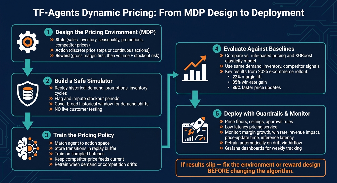
TF-Agents Dynamic Pricing: MDP Design to Deployment
Introduction to TF Agents and Deep Q Learning (Reinforcement learning with TensorFlow Agents)
sbb-itb-97f6a47
Design the Pricing Environment Before Training
Start by defining the MDP: state, action, and reward. Get any one of those wrong, and the policy learns the wrong pricing rule.
State design: demand, inventory, time, and competition
The state should include recent sales, inventory levels, seasonality, promotion history, and competitor prices.
- Recent sales - captures current demand momentum and short-term trend direction
- Inventory levels - prevents the agent from ignoring stockout risk when setting prices
- Seasonality - reflects recurring demand patterns tied to time of year or promotional calendar
- Promotion history - separates organic demand from promotion-driven spikes
- Competitor prices - anchors the agent's decisions to actual market conditions
One practical note on time zones: if your sales data mixes Eastern and Pacific timestamps without normalization, your day-of-week and hour-of-day features will get noisy. Standardize timestamps first. Then derive local-time features where needed.
Price elasticity is a derived feature, not a raw state variable. If the policy uses it as an input, label it that way and compute it upstream before passing it into the observation vector.
These inputs form the observation vector the agent sees at each pricing step.
Action space and reward rules
Use discrete price steps for simpler catalogs. Use continuous actions when you need finer control across many SKUs. Set reward around gross margin first, then volume and stockout risk.
Once the action space and reward are fixed, the simulator can enforce the same constraints during training.
Build a safe simulator with historical demand data
Do not test price changes on live customers. Build a simulator that replays historical demand, promotions, and inventory cycles so the agent can learn offline before deployment. The simulator needs to reproduce the same inventory limits, competitor response, and stockout behavior encoded in the reward.
Two simulator pitfalls need attention early. First, stockouts hide true demand and distort elasticity estimates. Flag stock-out periods, then impute or exclude them. Second, demand patterns shift. Promotions and market changes can alter how buyers respond, so the simulator should cover a broad enough historical window to capture those transitions.
With the environment defined, the next step is choosing the agent, replay buffer, and training loop.
Train a Pricing Policy with TF-Agents
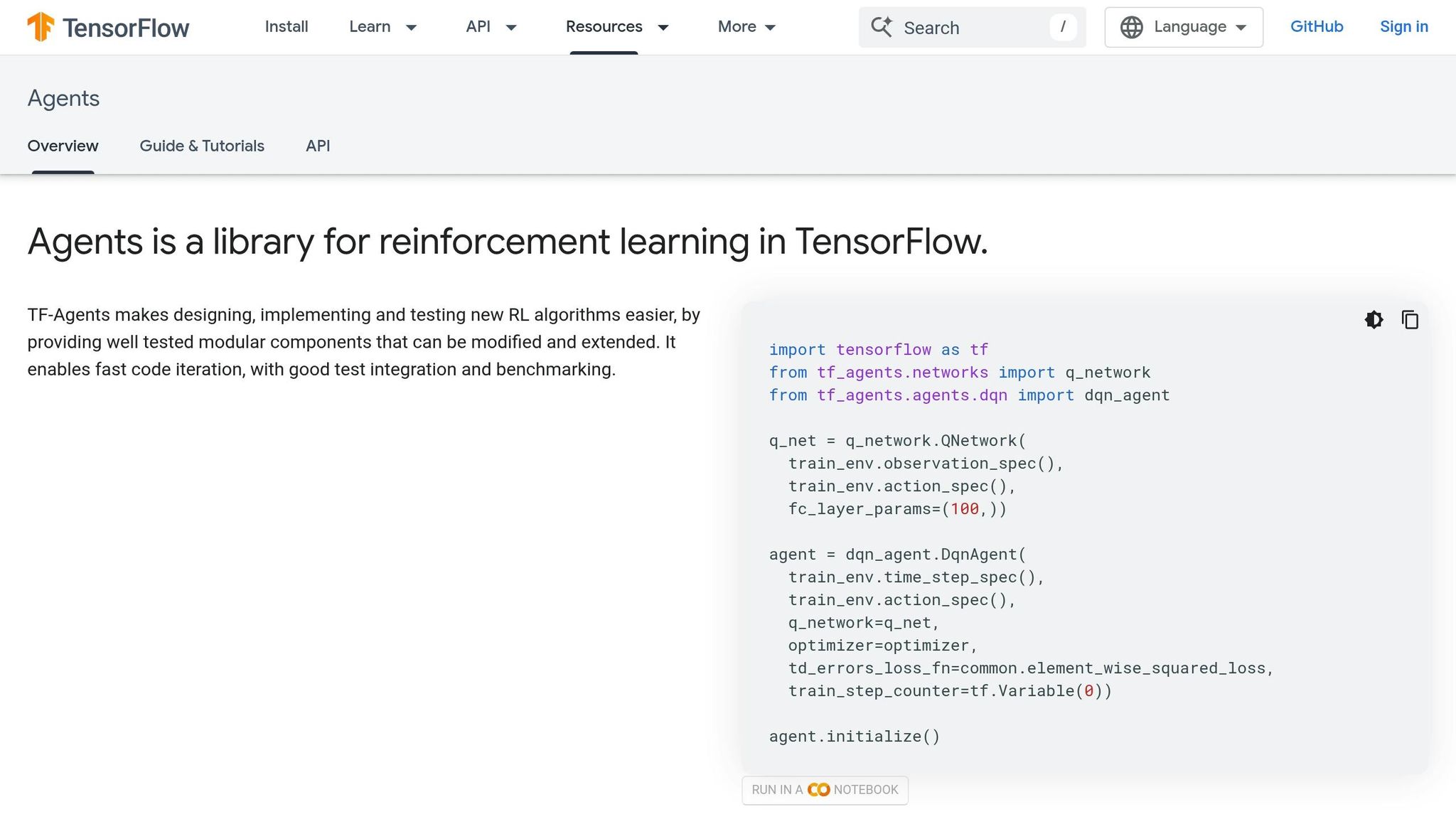
Choose the right agent for your pricing problem
Start by matching the agent to the action space. If price moves happen in fixed increments, use discrete actions. If you need tighter control, use continuous actions. Keep the first version simple and make sure it stays within inventory limits.
Once the action space is set, move on to data collection and policy learning.
Set up data collection, replay buffers, and training loops
After you pick the agent, the next step is generating training data and sampling it in a way the model can learn from. Train on simulator transitions built from historical sales, inventory, and competitor data. Then use that simulator to backtest policies before anything goes live.
Add forecast features only if they improve the demand signal. If they don't help, they just add noise. Store transitions in a replay buffer and train on sampled batches. Keep competitor-price feeds current, and retrain automatically when demand or competition drifts.
Control exploration cost and tune for stability
Start exploration in simulation, not in production. Then move to shadow-mode testing, where the policy produces decisions that are logged but not executed. That gives you a safe way to run A/B comparisons against the current policy without financial risk.
Stay in simulation or shadow mode until repeated runs show stable margin and win-rate lift.
Once exploration is under control, test the policy against baselines and offline evidence.
Evaluate, Deploy, and Monitor the Policy
Test against baselines and offline evidence
After offline training, validate the policy against clear baselines before anything goes live. Put it side by side with rule-based pricing and an XGBoost elasticity model, using the same demand, inventory, and competitor signals already defined in the simulator. That keeps the comparison fair and makes it easier to see whether the policy is adding value or just behaving differently.
Use the simulator to test candidate policies offline, then compare each model’s output against the rule-based and elasticity baselines.
"Static pricing rules did not account for demand trends or inventory constraints." - BuildNexTech
In one 2025 e-commerce rollout, pre-deployment testing showed a 22% margin lift and a 35% win rate gain.
Roll out with guardrails in production
If the offline results hold up, move the policy into production behind pricing guardrails. Run it through a low-latency pricing service and set hard limits with price floors, ceilings, and approval rules before a broader rollout.
That way, price updates stay in line with business rules and compliance requirements, even when the policy reacts to changing market conditions.
Monitor drift, retrain, and report business impact
Once the policy is live, keep watching the same signals used during training. Focus on drift in elasticity, demand, and competitor response. If those signals start to shift, retrain the policy with new sales logs and updated demand curves. Airflow can automate that retraining workflow.
For executive reporting, keep the scorecard simple and tied to business results:
- Margin growth
- Win rate
- Revenue impact
- Price-update time
- Inference latency
Use Grafana dashboards to track weekly performance and drift.
Common Mistakes and When to Bring in Outside Help
If results slip in production, check the setup before you blame the model.
Mistakes that derail TF-Agents pricing projects
When a policy misses the mark, the problem is usually upstream - in the state, reward, simulator, or governance. In plain English, most pricing failures start with setup mistakes.
A narrow state space gives the policy only part of the story. That means it learns from an incomplete view of the business. And if the reward pushes sales volume instead of profit margin and price elasticity, the agent may lift revenue while quietly eating into margin.
Misalignment across teams causes a different kind of trouble. If finance, product, and legal don't agree on KPIs before training begins, the project can drift fast. One team may want volume, another margin, and another risk control. At that point, the policy is being judged by three scorecards at once.
| Mistake | Business Consequence |
|---|---|
| Reward misaligned with margin | Optimizes volume at the expense of profitability |
| Unrealistic simulator | Leads to costly live failures |
| Missing shared KPI agreement | Conflicting success criteria across finance, product, and legal |
The result is margin leakage, weak seasonal response, and poor elasticity visibility.
When consulting support makes sense
Things get harder fast when pricing has to work across many SKUs and disconnected data sources. Outside help makes sense when pricing covers thousands of SKUs, needs sub-50 ms inference, or depends on siloed sales, demand, inventory, and competitor feeds.
Some teams just don't have the time or bench to build production-grade MDP design, simulation engineering, and deployment guardrails in-house. In those cases, the Top Consulting Firms Directory lists firms by category.
Conclusion: What to build first and what to measure
Start with one product category. Keep the state space narrow, reward margin and elasticity, and train offline in a historical-data simulator.
Then track the metrics that matter:
- Revenue
- Gross margin
- Elasticity
- Pricing turnaround time
If those numbers stall, fix the environment or reward design before changing the algorithm. That keeps attention on the setup instead of over-tuning the model.
FAQs
When is RL better than static pricing?
RL beats static, rules-based pricing when you’re dealing with large catalogs, fast-moving market shifts, or messy inputs like price elasticity and competitor moves.
Static rules still make sense for stable catalogs with fewer than 200 SKUs or in regulated settings. But as things get more dynamic, RL has the edge. It can scale across many products and adjust in real time when demand jumps, inventory shifts, or competitors change prices.
How much historical data do I need?
Before launching the model, audit transaction-level data from the past 2 to 4 weeks. The goal is simple: make sure the data is complete, reliable, and shows steady price variation. If that check is weak, the model starts on shaky ground.
For A/B testing and training, run experiments for at least 2 to 4 weeks. Also aim for 200 conversions per variant so you can pick up dependable demand signals.
What should I fix first if results drop?
First, check your data quality and consistency. Audit transaction-level data to make sure it’s complete, reliable, and shows steady price variation.
Also look for training-serving skew, where the features used at inference differ from the ones used in training. And make sure model monitoring can catch anomalies before they bury the root cause.